Write down your research question (from component 1)
How does the number of coaches assigned to US college sports teams vary by the gender of the team?
Write down your hypothesis (from component 1)
I predict that for sports in which there is both a men’s and a women’s team, coaching levels will be equivalent. I expect this because universities are required to adhere to Title IX, which would prohibit different levels of resources for equivalent sports.
Write down the name of your data set (from component 1)
Write down the names of the variables you will use in your analysis (i.e., what you need to type to access them in R)
ncoaches, teamgender, sport
For each variable, write:
A brief description of what it measures
Whether it is an explanatory (independent) variable, a response (dependent) variable, or something else (explain what)
What kind of variable it is (categorical or numeric and which subtype within these)
ncoaches: This measures the number of coaches on each team. It is my response variable. It is a discrete numeric variable.
teamgender: This records the gender of the players on the team. It is an explanatory variable and it is nominal categorical.
sport: I will use this variable to limit my data frame to the sports that have both men’s and women’s teams. It is a nominal categorical variable.
Part 2: Univariate distributions
For each of your variables:
Look at its distribution using the summary() or table() function (as appropriate to its type).
Indicate how many missing values (NAs) there are.
In ~2-3 sentences, describe what you see in the results. Note anything that surprises you.
ncoaches:
The minimum number of coaches per team is one, the median is four, and the maximum is 14. There are no missing values. The fourth quartile is much wider than the other three (spanning from 4-14), and the mean (3.9) is larger than the median, suggesting that the data may be skewed to the right. In other words, there may be a small number of teams with a large number of coaches relative to the rest.
The median and the cutoff point for the third quartile are the same (both equal 4), indicating that four is a really common number of coaches for teams to have.
summary(sports$ncoaches)
   Min. 1st Qu.  Median    Mean 3rd Qu.    Max.
  1.000   3.000   4.000   4.058   4.000  14.000
teamgender:
There are 418 men’s teams and 461 women’s teams in these data. There are no missing values. I am surprised that there are so many more women’s teams than men’s teams. I would have expected the numbers to be about the same.
table(sports$teamgender, useNA ="always")
  men women  <NA>
  418   461     0
sport:
There are 17 sports represented in my data (though it is likely that “All Track Combined” and “Track and Field X Country” are different words for the same thing, which would make it 16 sports). There are no missing values. Most sports have either 76 or 38 distinct teams in my data. It is possible that the sports with 38 teams are those that are available only to one gender, and the ones with 76 (38x2) teams have both men’s and women’s versions.
table(sports$sport, useNA ="always")
       All Track Combined                  Baseball                Basketball
                       72                        38                        76
                  Fencing              Field Hockey                  Football
                       76                        38                        38
                     Golf                Gymnastics                  Lacrosse
                       76                        19                        76
                   Rowing                    Soccer                  Softball
                       38                        76                        24
      Swimming and Diving                    Tennis Track and Field X Country
                       76                        76                         4
               Volleyball                 Wrestling                      <NA>
                       38                        38                         0
Part 3: Preparing your data set
Will you analyze all the observations in your data set? Explain why or why not. If not, which will you include and which will you exclude?
I will not analyze all of the observations in my data set because analyzing all of them would make for an unfair comparison. There is a different set of sports available for men than for women. I am interested in comparing the number of coaches for comparable men’s and women’s teams, so I will exclude sports for which there are only men’s teams or only women’s teams (e.g., football, softball).
Do you need to create any new variables? Explain why or why not. If so, what are they?
I do not need to create any new variables. My explanatory variable is teamgender and my response variable is ncoaches, and they already fit my research question well in their current forms.
If necessary, use the code chunk below to make any needed changes (filtering observations and creating variables) to your data.
# first, I need to figure out which sports have teams for both genderstable(sports$sport, sports$teamgender)
                            men women
  All Track Combined         36    36
  Baseball                   38     0
  Basketball                 38    38
  Fencing                    38    38
  Field Hockey                0    38
  Football                   38     0
  Golf                       38    38
  Gymnastics                  0    19
  Lacrosse                   38    38
  Rowing                      0    38
  Soccer                     38    38
  Softball                    0    24
  Swimming and Diving        38    38
  Tennis                     38    38
  Track and Field X Country   2     2
  Volleyball                  0    38
  Wrestling                  38     0
# from that table, I can see that I need to remove baseball, field hockey, football, gymnastics, rowing, softball, volleyball, and wrestling.sports_filtered <- sports |>filter( sport !="Baseball", sport !="Field Hockey", sport !="Football", sport !="Gymnastics", sport !="Rowing", sport !="Softball", sport !="Volleyball", sport !="Wrestling" )# did it work? Let's make the same table with the new data settable(sports_filtered$sport, sports_filtered$teamgender)
                            men women
  All Track Combined         36    36
  Basketball                 38    38
  Fencing                    38    38
  Golf                       38    38
  Lacrosse                   38    38
  Soccer                     38    38
  Swimming and Diving        38    38
  Tennis                     38    38
  Track and Field X Country   2     2
# now all the sports have both men's and women's teams--we're good to go!
Part 4: Multivariate visualizations
Make a plot showing the relationship between your explanatory (independent) and response (dependent) variables. Depending on your variable types, this might be a scatter plot, box plot, bar chart, etc. Include meaningful axis labels.
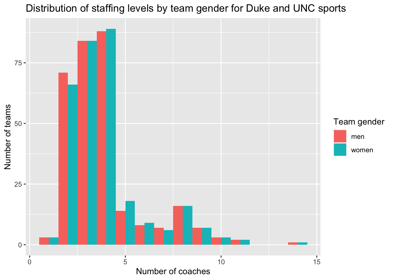
Interpret your plot in a few sentences. Does it appear these variables are associated with one another? Does anything about the relationship surprise you? Is it consistent or inconsistent with your hypothesis?
As suggested by the univariate summary statistics, the distribution of the number of coaches is skewed to the right. The distributions look nearly identical for men’s and women’s teams, so it appears that team gender and staffing levels are probably not associated with one another. This is consistent with my hypothesis and is not very surprising, though I was not expecting the distributions to be as extraordinarily similar as they appear here.
# I have one numeric and one categorical variable, so a boxplot (as in example code in the assignment template) would also be a good choice here--but for variety I will show the same information in histogram formggplot(data = sports_filtered, aes(x = ncoaches, fill = teamgender)) +geom_histogram(position =position_dodge(), # this puts the bars next to each otherbinwidth =1 ) +labs(x ="Number of coaches",y ="Number of teams",title ="Distribution of staffing levels by team gender for Duke and UNC sports",fill ="Team gender")