Describing data: part 2

Lecture 8

Aidan Combs

Duke University
SOCIOL 333 - Summer Term 1 2023

2023-05-31

Logistics

Project proposals
- I will get my feedback to you soon–will be posted as a github issue (grades will be in Sakai)

Project descriptive statistics
- Due Tuesday June 6. Instructions are up; template and example to come this afternoon.

Homework 1
- Cancelled as a mandatory assignment; time is short
- BUT practice is the only way to learn this stuff!
- So, extra credit opportunities will be worked into exercises–I highly recommend doing as much as you can!

Today

Finish univariate summaries
Preparing data frames

Where we left off: summarizing numeric variables

Summarizing a distribution

Center
- median(dataset$var, na.rm = TRUE)
- mean(dataset$var, na.rm = TRUE)
Spread
- quantile(dataset$var, na.rm = TRUE)
- sd(dataset$var, na.rm = TRUE)
(Almost) everything
- summary(dataset$var)

Exercise question 2

glimpse(acs12)

Rows: 2,000
Columns: 13
$ income       <int> 60000, 0, NA, 0, 0, 1700, NA, NA, NA, 45000, NA, 8600, 0,…
$ employment   <fct> not in labor force, not in labor force, NA, not in labor …
$ hrs_work     <int> 40, NA, NA, NA, NA, 40, NA, NA, NA, 84, NA, 23, NA, NA, N…
$ race         <fct> white, white, white, white, white, other, white, other, a…
$ age          <int> 68, 88, 12, 17, 77, 35, 11, 7, 6, 27, 8, 69, 69, 17, 10, …
$ gender       <fct> female, male, female, male, female, female, male, male, m…
$ citizen      <fct> yes, yes, yes, yes, yes, yes, yes, yes, yes, yes, yes, ye…
$ time_to_work <int> NA, NA, NA, NA, NA, 15, NA, NA, NA, 40, NA, 5, NA, NA, NA…
$ lang         <fct> english, english, english, other, other, other, english, …
$ married      <fct> no, no, no, no, no, yes, no, no, no, yes, no, no, yes, no…
$ edu          <fct> college, hs or lower, hs or lower, hs or lower, hs or low…
$ disability   <fct> no, yes, no, no, yes, yes, no, yes, no, no, no, no, yes, …
$ birth_qrtr   <fct> jul thru sep, jan thru mar, oct thru dec, oct thru dec, j…

Question 2 solutions

What is the mean of hrs_work? What is the median? (there are two ways to get this info)

Approach 1:

mean(acs12$hrs_work, na.rm = TRUE)

[1] 37.97706

median(acs12$hrs_work, na.rm = TRUE)

[1] 40

Approach 2:

summary(acs12$hrs_work)

   Min. 1st Qu.  Median    Mean 3rd Qu.    Max.    NA's 
   1.00   32.00   40.00   37.98   40.00   99.00    1041

Question 2 solutions

What is the standard deviation of hrs_work?

sd(acs12$hrs_work, na.rm = TRUE)

[1] 13.49768

Question 2 solutions

What proportion of people in the data set are missing information (have NAs) for this variable? (there are many ways to do this)

# Find the number of NA values
summary(acs12$hrs_work)

   Min. 1st Qu.  Median    Mean 3rd Qu.    Max.    NA's 
   1.00   32.00   40.00   37.98   40.00   99.00    1041

# Find the total number of observations
glimpse(acs12)

Rows: 2,000
Columns: 13
$ income       <int> 60000, 0, NA, 0, 0, 1700, NA, NA, NA, 45000, NA, 8600, 0,…
$ employment   <fct> not in labor force, not in labor force, NA, not in labor …
$ hrs_work     <int> 40, NA, NA, NA, NA, 40, NA, NA, NA, 84, NA, 23, NA, NA, N…
$ race         <fct> white, white, white, white, white, other, white, other, a…
$ age          <int> 68, 88, 12, 17, 77, 35, 11, 7, 6, 27, 8, 69, 69, 17, 10, …
$ gender       <fct> female, male, female, male, female, female, male, male, m…
$ citizen      <fct> yes, yes, yes, yes, yes, yes, yes, yes, yes, yes, yes, ye…
$ time_to_work <int> NA, NA, NA, NA, NA, 15, NA, NA, NA, 40, NA, 5, NA, NA, NA…
$ lang         <fct> english, english, english, other, other, other, english, …
$ married      <fct> no, no, no, no, no, yes, no, no, no, yes, no, no, yes, no…
$ edu          <fct> college, hs or lower, hs or lower, hs or lower, hs or low…
$ disability   <fct> no, yes, no, no, yes, yes, no, yes, no, no, no, no, yes, …
$ birth_qrtr   <fct> jul thru sep, jan thru mar, oct thru dec, oct thru dec, j…

Question 2 solutions

Now that we have those values, we can use R to do the math

# Divide!
1041/2000

[1] 0.5205

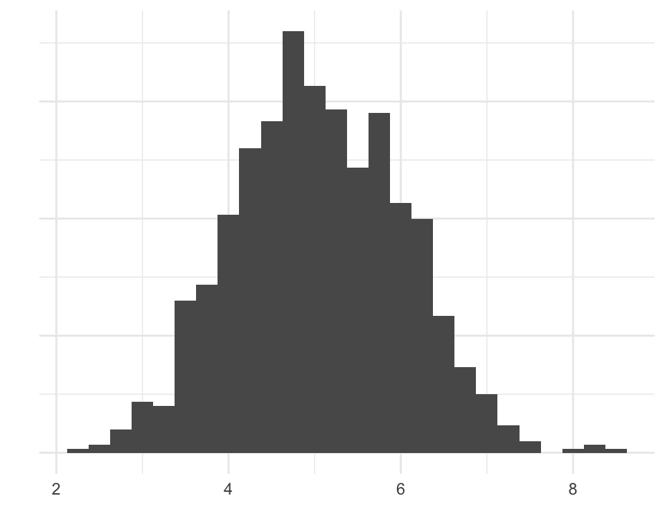
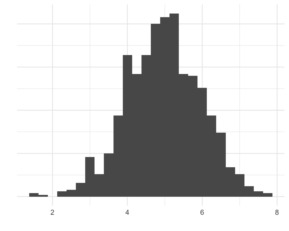
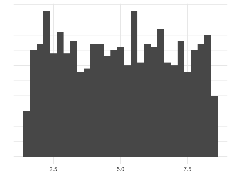
Shape

We’ll go over how to make plots later
But summary statistics tell you things about shape too

Skew

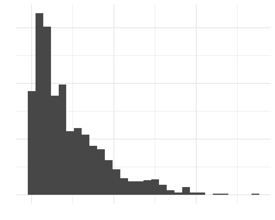
Right-skewed data

Left-skewed data

Skew

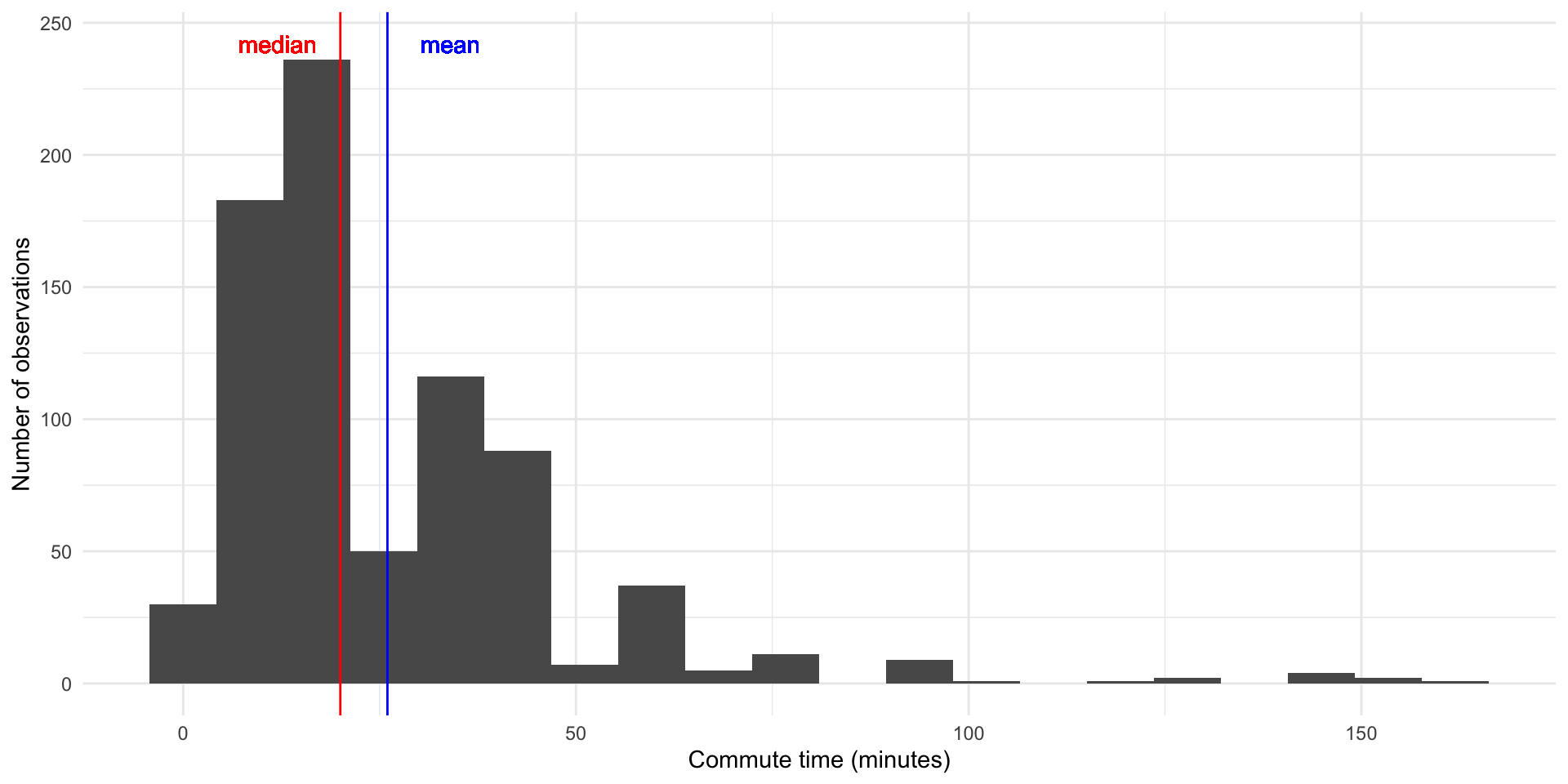
Extreme values influence the mean more than the median
When mean is higher than median: data might be skewed right (and vice versa)

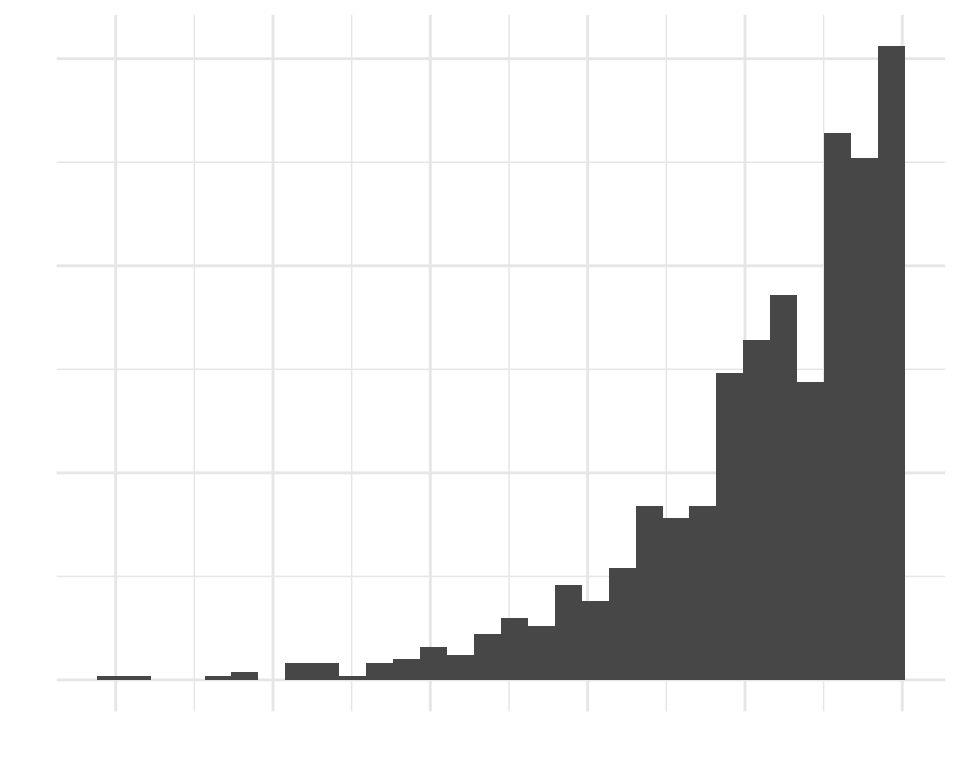
Example: American Community Survey commute time

time_to_work: Travel time to work, in minutes.

mean_commute <- mean(acs12$time_to_work, na.rm = TRUE)
median_commute <- median(acs12$time_to_work, na.rm = TRUE)

mean_commute

[1] 25.99745

median_commute

[1] 20

Example: American Community Survey commute time

Shape: Quartiles

Location of quartiles also tells you something about shape

summary(acs12$time_to_work)

   Min. 1st Qu.  Median    Mean 3rd Qu.    Max.    NA's 
      1      10      20      26      30     163    1217

Review

Categorical data: look at the available categories and how many observations are in each category
- unique(dataframe$variable)
- table(dataframe$variable, useNA = "always")
- table(dataframe$variable1, dataframe$variable2, useNA = "always")

Review

Numeric data: Look at summary statistics that tell you something about the distribution
- summary(dataframe$variable)
- sd(dataframe$variable, na.rm = TRUE)

Modifying data frames

Removing observations

You may not be interested in all observations
Example:
- RQ: How is commute time related to hours worked?

Removing observations

How is commute time related to hours worked?
Data: ACS 2012

glimpse(acs12)

Rows: 2,000
Columns: 13
$ income       <int> 60000, 0, NA, 0, 0, 1700, NA, NA, NA, 45000, NA, 8600, 0,…
$ employment   <fct> not in labor force, not in labor force, NA, not in labor …
$ hrs_work     <int> 40, NA, NA, NA, NA, 40, NA, NA, NA, 84, NA, 23, NA, NA, N…
$ race         <fct> white, white, white, white, white, other, white, other, a…
$ age          <int> 68, 88, 12, 17, 77, 35, 11, 7, 6, 27, 8, 69, 69, 17, 10, …
$ gender       <fct> female, male, female, male, female, female, male, male, m…
$ citizen      <fct> yes, yes, yes, yes, yes, yes, yes, yes, yes, yes, yes, ye…
$ time_to_work <int> NA, NA, NA, NA, NA, 15, NA, NA, NA, 40, NA, 5, NA, NA, NA…
$ lang         <fct> english, english, english, other, other, other, english, …
$ married      <fct> no, no, no, no, no, yes, no, no, no, yes, no, no, yes, no…
$ edu          <fct> college, hs or lower, hs or lower, hs or lower, hs or low…
$ disability   <fct> no, yes, no, no, yes, yes, no, yes, no, no, no, no, yes, …
$ birth_qrtr   <fct> jul thru sep, jan thru mar, oct thru dec, oct thru dec, j…

-   Need to remove people who are unemployed/not in labor force (and don't have a job or a commute!)

Removing observations

How? With filter()
filter(dataframe, condition)

acs12_employedonly <- filter(acs12, employment == "employed")

Did it work? Check with table()

table(acs12_employedonly$employment, useNA = "always")


not in labor force         unemployed           employed               <NA> 
                 0                  0                843                  0

Conditions

filter(acs12, employment == "employed")
condition: employment == "employed"
This specifies which observations you want to keep

Common comparison operators:
- == : equal to (note there are two equals signs!)
- != : not equal to
- >, >= : greater than, greater than or equal to
- <, <= : less than, less than or equal to

Values:
- Can be numbers, letters/words, or TRUE/FALSE–should match the response options of your variable
- Put letters/words in quotation marks

Condition examples

filter(acs12, citizen == "no")
filter(acs12, income <= 12000)
filter(acs12, birth_qrtr != "jan thru mar")
filter(acs12, hrs_work > 20)

Other useful condition operators

Two or more requirements
- & : and
- | : or
- filter(acs12, citizen == "no" & lang == "english")
- filter(acs12, race == "black" | race == "asian")
Missing values
- is.na()
- !is.na()
  - is not missing – good for removing rows with missing values
- filter(acs12, !is.na(income))
More: Click here for R for Data Science

Common mistakes and error messages

filter(acs12, employment = "employed")

Error in `filter()`:
! We detected a named input.
ℹ This usually means that you've used `=` instead of `==`.
ℹ Did you mean `employment == "employed"`?

Common mistakes and error messages

filter(acs12, employment == employed)

Error in `filter()`:
ℹ In argument: `employment == employed`.
Caused by error:
! object 'employed' not found

Common mistakes and error messages

filter(acs12, employment == "employd")

# A tibble: 0 × 13
# ℹ 13 variables: income <int>, employment <fct>, hrs_work <int>, race <fct>,
#   age <int>, gender <fct>, citizen <fct>, time_to_work <int>, lang <fct>,
#   married <fct>, edu <fct>, disability <fct>, birth_qrtr <fct>

Common mistakes and error messages

filter(acs12, employment == "Employed")

# A tibble: 0 × 13
# ℹ 13 variables: income <int>, employment <fct>, hrs_work <int>, race <fct>,
#   age <int>, gender <fct>, citizen <fct>, time_to_work <int>, lang <fct>,
#   married <fct>, edu <fct>, disability <fct>, birth_qrtr <fct>

Exercise: Filtering

Clone and open the project repo now (ex-5-31-yourusername)
Then open the .qmd file and try out some filtering
- Instructions: Computing -> Cloning and committing