Describing data: part 1

Lecture 7

Aidan Combs

Duke University
SOCIOL 333 - Summer Term 1 2023

2023-05-30

Logistics

• Final project proposals due tonight

  • Update your first draft: incorporate useful peer feedback
  • Don’t forget to add the last paragraph about what question you think you should go with
  • Any last questions?

• Late work policy

  • You have 3 no-questions-asked late days to use through the semester
  • Applies to project components and assignments (except final paper and presentation–I can’t extend those)

Today

• Data analysis process
• Univariate summaries: what do my variables look like?

The (approximate) data analysis process

• Determine topic
• Find data; learn what observations and variables are available
• Write research question
• Describe distributions of relevant variables
• Prepare data frame for analysis
• Describe relationships between variables
• Perform statistical tests/write models
• Communicate results

The (approximate) data analysis process

• Determine topic ✓
• Find data; learn what observations and variables are available ✓
• Write research question ✓
• Describe distributions of relevant variables
• Prepare data frame for analysis
• Describe relationships between variables
• Perform statistical tests/write models
• Communicate results

The (approximate) data analysis process

• Determine topic ✓
• Find data; learn what observations and variables are available ✓
• Write research question ✓
• Describe distributions of relevant variables
• Prepare data frame for analysis
• Describe relationships between variables
• Perform statistical tests/write models
• Communicate results

Project component 2: Descriptive statistics

Goals:

• Understand how your variables are distributed in your data

• Make any necessary modifications to your data frame

  • Remove irrelevant observations
  • Modify or create variables as necessary

• Describe the relationships between your variables

Understanding how your variables are distributed

Today: With numbers (later: with plots)

• Summary statistics
• What makes sense depends on variable type

R syntax for today

• To access specific variables: dataframe$variable
• Functions do things with variables/other inputs: do_this(with_this)
• We can save results as objects to use later with <-: an_object_name <- some_function(some_input)
  • eg: meanvalue <- mean(dataframe$variable)

Data set 1 for today: EADA data on sports teams

glimpse(sports)

Rows: 879
Columns: 8
$ school             <chr> "Duke", "Duke", "Duke", "Duke", "Duke", "Duke", "Du…
$ year               <dbl> 2003, 2003, 2003, 2003, 2003, 2003, 2003, 2003, 200…
$ division           <chr> "NCAA Division I-A", "NCAA Division I-A", "NCAA Div…
$ teamgender         <chr> "men", "men", "men", "men", "men", "men", "men", "m…
$ sport              <chr> "Baseball", "Basketball", "Fencing", "Football", "G…
$ ncoaches           <dbl> 3, 4, 1, 10, 2, 3, 3, 2, 2, 3, 3, 4, 4, 8, 6, 13, 2…
$ nplayers           <dbl> 33, 15, 19, 81, 12, 45, 23, 32, 11, 50, 35, 35, 30,…
$ player_coach_ratio <dbl> 11.000000, 3.750000, 19.000000, 8.100000, 6.000000,…

Before we dive in: an intro to missing data

• Sometimes not everyone answers every question or data is not available for a specific observation
• Creates NA values in your data frame
• Check for them–they can create unexpected results otherwise

Categorical variables

Categorical: What are the options?

• unique()

unique(sports$school)

[1] "Duke" "UNC" 

unique(sports$sport)

 [1] "Baseball"                  "Basketball"               
 [3] "Fencing"                   "Football"                 
 [5] "Golf"                      "Lacrosse"                 
 [7] "Soccer"                    "Swimming and Diving"      
 [9] "Tennis"                    "Track and Field X Country"
[11] "Wrestling"                 "All Track Combined"       
[13] "Field Hockey"              "Rowing"                   
[15] "Volleyball"                "Gymnastics"               
[17] "Softball"                 

Categorical: counts for one variable

• Counts: table()

  • useNA = "always" tells R to let you know if there is any missing data on your variables

table(sports$school, useNA = "always")

Duke  UNC <NA> 
 423  456    0 

Categorical: counts for two variables

• Still table(), but use two variables as arguments

table(sports$teamgender, sports$school, useNA = "always")

       
        Duke UNC <NA>
  men    209 209    0
  women  214 247    0
  <NA>     0   0    0

Exercise

• Today’s exercise: in R! Clone and open the project repo now (ex-5-30-yourusername)

  • Instructions: Computing -> Cloning and committing

• Data: American Community Survey 2012

glimpse(acs12)

Rows: 2,000
Columns: 13
$ income       <int> 60000, 0, NA, 0, 0, 1700, NA, NA, NA, 45000, NA, 8600, 0,…
$ employment   <fct> not in labor force, not in labor force, NA, not in labor …
$ hrs_work     <int> 40, NA, NA, NA, NA, 40, NA, NA, NA, 84, NA, 23, NA, NA, N…
$ race         <fct> white, white, white, white, white, other, white, other, a…
$ age          <int> 68, 88, 12, 17, 77, 35, 11, 7, 6, 27, 8, 69, 69, 17, 10, …
$ gender       <fct> female, male, female, male, female, female, male, male, m…
$ citizen      <fct> yes, yes, yes, yes, yes, yes, yes, yes, yes, yes, yes, ye…
$ time_to_work <int> NA, NA, NA, NA, NA, 15, NA, NA, NA, 40, NA, 5, NA, NA, NA…
$ lang         <fct> english, english, english, other, other, other, english, …
$ married      <fct> no, no, no, no, no, yes, no, no, no, yes, no, no, yes, no…
$ edu          <fct> college, hs or lower, hs or lower, hs or lower, hs or low…
$ disability   <fct> no, yes, no, no, yes, yes, no, yes, no, no, no, no, yes, …
$ birth_qrtr   <fct> jul thru sep, jan thru mar, oct thru dec, oct thru dec, j…

Question 1 solutions

Response options for the employment variable

unique(acs12$employment)

[1] not in labor force <NA>               employed           unemployed        
Levels: not in labor force unemployed employed

Question 1 solutions

How many people are in each category? How many missing values are there?

table(acs12$employment, useNA = "always")

not in labor force         unemployed           employed               <NA> 
               656                106                843                395 

Question 1 solutions

Create a table that shows the number of people of each gender in each employment category.

table(acs12$gender, acs12$employment, useNA = "always")

        
         not in labor force unemployed employed <NA>
  male                  283         59      470  219
  female                373         47      373  176
  <NA>                    0          0        0    0

Does it look like gender and employment status are related?

Numeric variables

Numeric: All about distributions!

Summarizing a distribution

• Center
• Spread
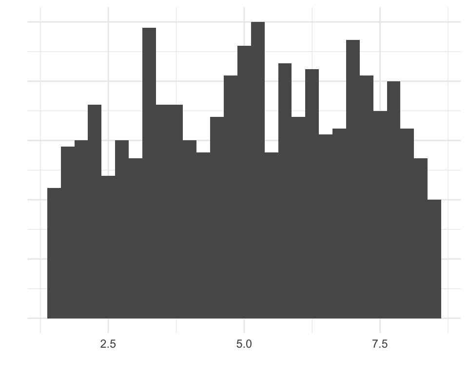
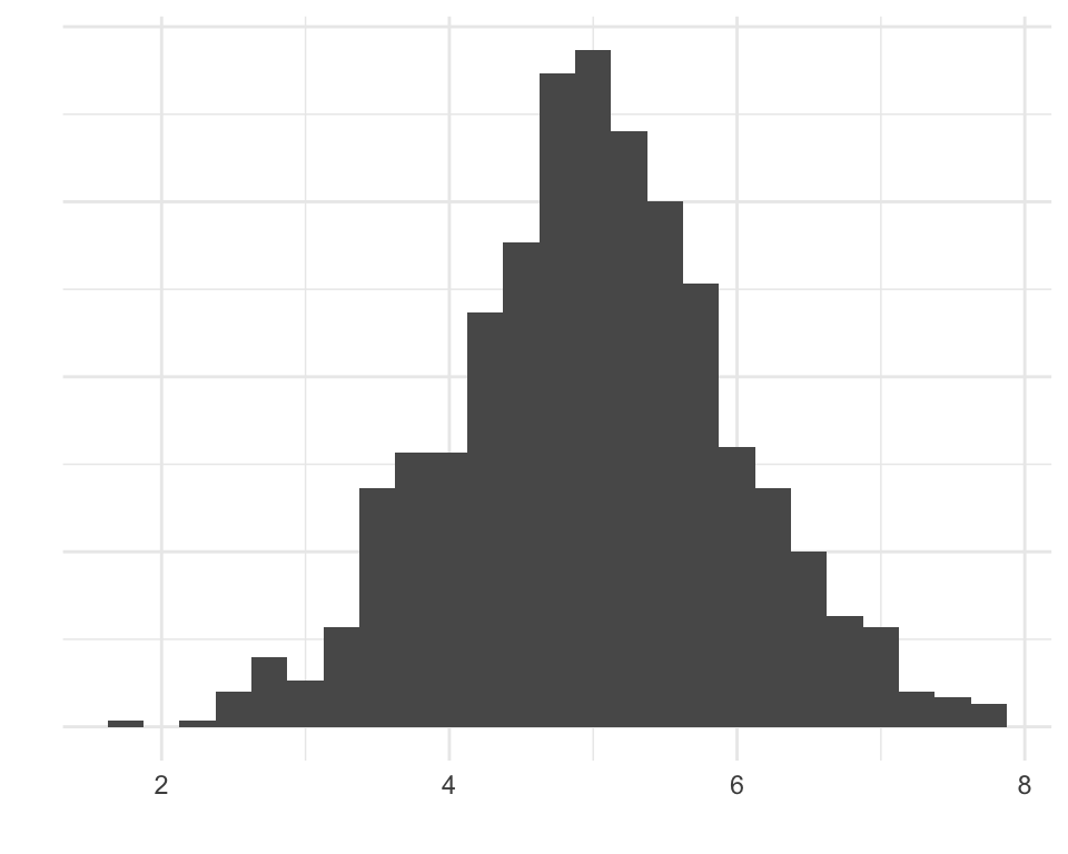
• Shape

Center: Mean

Say we measure heights of 7 people (in inches):

heights <- c(67, 70, 80, 61, 70, 71, 62)

• aka the average
• Add everything together and divide by the number of values: (66 + 70 + 80 + 62 + 68 + 71 + 62)/7 = 68.7
• mean()

mean(heights)

[1] 68.71429

Center: Median

heights

[1] 67 70 80 61 70 71 62

• The middle value
• Order the values least to greatest, select the one in the middle
• 61, 62, 67, 70, 70, 71, 80
• median()

median(heights)

[1] 70

Spread: minimum and maximum

min(heights)

[1] 61

max(heights)

[1] 80

Spread: quartiles

• percentiles
• lowest 1/4 of your data is below the 25th percentile, lowest 1/2 below 50%, etc
• Calculated similarly to the median
• quantile()

quantile(heights)

  0%  25%  50%  75% 100% 
61.0 64.5 70.0 70.5 80.0 

Spread: standard deviation

• Measure of degree of variation in data: bigger standard deviation = more variation
• Used to establish statistical significance–we’ll come back to this later
• sd()

heights_moresimilar <- c(60, 63, 62, 60, 61, 61, 64)

heights

[1] 67 70 80 61 70 71 62

heights_moresimilar

[1] 60 63 62 60 61 61 64

sd(heights)

[1] 6.369571

sd(heights_moresimilar)

[1] 1.511858

summary(): (almost) everything all at once

summary(sports$nplayers)

   Min. 1st Qu.  Median    Mean 3rd Qu.    Max. 
   5.00   15.00   28.00   35.63   40.00  148.00 

Summary statistics functions and missing values

mean(acs12$income)

[1] NA

• NA! What!

• Summary statistics functions will return NA if any of the observations are missing information for the variable
• Always check for missing data!
• Use the na.rm = TRUE option to tell the function to ignore the NA values.

summary(acs12$income)

   Min. 1st Qu.  Median    Mean 3rd Qu.    Max.    NA's 
      0       0    3000   23600   33700  450000     377 

mean(acs12$income, na.rm = TRUE)

[1] 23599.98