Hypothesis tests pt 3

Lecture 15

Aidan Combs

Duke University
SOCIOL 333 - Summer Term 1 2023

2023-06-13

Logistics

• Project component 3, results: draft by Thursday (June 15), submit for grading next Tuesday (June 20)

  • Drafts should be complete–meaning you attempted all parts
  • Instructions and example are posted

Today

• Selecting the correct hypothesis test
• Running hypothesis tests in infer

Different types of tests

• To figure out what test you need, you need to know some things about your variables:

  • What is/are your explanatory variable(s)? What type of variable is it/are they (categorical with two levels, categorical with three levels, or numeric)? How many explanatory variables are there?
  • What is your response variable? What type of variable is it?

A recap on variables

• They never go away! Identifying what kind of variables you have and what role they’re playing in your analysis is really central. Here’s a summary of the distinctions that are relevant here.

A recap on variables: types

• Numeric. The responses are numbers

  • Income, height, age

• Categorical with two categories: The response options are categories–represented with words, not (meaningful) numeric values. There are only two response options available. This includes binary variables.

  • Sex assigned at birth (male/female), married or not, hired or not

• Categorical with three or more categories: The response options are categories, like above, but there are more than two possibilities.

  • Race, smoking status (never, current, former), music genre preference

A recap on variables: roles in your analysis

• Explanatory/independent: The thing doing the explaining; the thing that comes first
• Response/dependent: The outcome that is being predicted; the thing that comes second, possibly as a result of the explanatory variable.

A recap on variables

• Example: How does whether a student attends a public or private high school affect their probability of graduating?

• What are the explanatory and response variables? What are their types?

  • Explanatory: Type of high school (public or private): categorical with two categories

  • Response: Graduated or not: categorical with two categories

    • Why not probability of graduating? Because we can’t observe that for any individual person. We observe whether each one graduated or not. Then we use that to calculate probabilities for the two groups in the sample: those at private high schools and those at public high schools.

Identifying the right test: exercise Q1

• This one is in R—find the ex-6-13-yourusername repo on GitHub and clone it

• For each research question, identify the explanatory variable, the response variable, their types, and the correct statistical test

  • Think about what the data would look like for each individual!

Identifying the right test: exercise Q1

Identifying the right test: exercise Q1

• a. How does the amount of money a country spends on healthcare (per person) affect its average life expectancy?

• Explanatory variable(s) and type(s)?

  • Amount of money per person a country spends on healthcare. Numeric.

• Response variable and type?

  • Average life expectancy. Numeric.

• Correct statistical test?

  • Linear regression

Identifying the right test: exercise Q2

• Same thing, new questions. For each one, identify the explanatory variable, the response variable, their types, and the correct statistical test

Identifying the right test: exercise Q2b

• How is a patient’s body mass index related to the probability a doctor refers them to a specialist?

• Explanatory variable(s) and type(s)?

  • Body mass index. Numeric.

• Response variable and type?

  • Whether or not they are referred to a specialist. Categorical with two categories (yes/no).

• Correct statistical test?

  • Logistic regression

Identifying the right test: exercise Q2c

• How do outcomes of traffic stops (which can be warnings, citations, or arrests) vary by the driver’s race?

• Explanatory variable(s) and type(s)?

  • Driver’s race. Categorical with three or more categories.

• Response variable and type?

  • Outcomes of traffic stops. Categorical with three or more categories.

• Correct statistical test?

  • Chi-square test of independence

We know what test we need! Now what?

Running a hypothesis test in R with infer

• The bad news: there are a lot of different tests.

• The good news: regardless of what specific test you run, the logic is similar, and your code will look about the same!

• We will be using the infer package to conduct hypothesis tests

  • infer is built to work on similar logic to the tidyverse—where filter(), mutate(), and ggplot() are from
  • Its documentation is excellent—check out the website (link here) if you ever get stuck. It has lots of examples of every kind of test it can run.

Steps to running a hypothesis test with infer

1. Calculate the test statistic of your sample
2. Simulate the null distribution
3. Calculate the p value of your sample
4. Visualize the test statistic of your sample alongside the null distribution

Step 1: Calculate the test statistic of your sample

• Test statistic: A number that quantifies how much your sample differs from the expected sampling distribution.
• For example: Z scores
• Different tests use different test statistics
• Regardless of what it is specifically, step 1 is to calculate it.

Step 1: Calculate the test statistic of your sample

• We’ll use the gss data (a nationally representative survey of American adults).

• Our question: How does the probability of obtaining a college degree vary by sex assigned at birth?

  • Explanatory variable: sex assigned at birth (categorical w two categories)
  • Response variable: Whether or not someone obtained a college degree (categorical w two categories)
  • So we’ll use a two sample Z test

glimpse(gss)

Rows: 500
Columns: 11
$ year    <dbl> 2014, 1994, 1998, 1996, 1994, 1996, 1990, 2016, 2000, 1998, 20…
$ age     <dbl> 36, 34, 24, 42, 31, 32, 48, 36, 30, 33, 21, 30, 38, 49, 25, 56…
$ sex     <fct> male, female, male, male, male, female, female, female, female…
$ college <fct> degree, no degree, degree, no degree, degree, no degree, no de…
$ partyid <fct> ind, rep, ind, ind, rep, rep, dem, ind, rep, dem, dem, ind, de…
$ hompop  <dbl> 3, 4, 1, 4, 2, 4, 2, 1, 5, 2, 4, 3, 4, 4, 2, 2, 3, 2, 1, 2, 5,…
$ hours   <dbl> 50, 31, 40, 40, 40, 53, 32, 20, 40, 40, 23, 52, 38, 72, 48, 40…
$ income  <ord> $25000 or more, $20000 - 24999, $25000 or more, $25000 or more…
$ class   <fct> middle class, working class, working class, working class, mid…
$ finrela <fct> below average, below average, below average, above average, ab…
$ weight  <dbl> 0.8960034, 1.0825000, 0.5501000, 1.0864000, 1.0825000, 1.08640…

Step 1.1: specify what your variables are

• How does the probability of obtaining a college degree vary by sex assigned at birth?
• First, we use specify() to tell R what variables we’re interested in

test_stat <- gss |>           # remember the pipe operator? It will be useful here!
  specify(explanatory = sex,
          response = college,
          success = "degree") # this last "success" piece is used for two sample Z tests only.
                              # it determines how the proportion is calculated (proportion of 
                              # people who have a degree, or proportion of people who don't)

Step 1.2: hypothesize to tell R what your null hypothesis is

• Then R needs to know what our null hypothesis is. Usually in this class, our null hypotheses will be that two variables are not related.
• We tell R this by adding hypothesize(null = "independence") to our pipeline

test_stat <- gss |> 
  specify(explanatory = sex,
          response = college,
          success = "degree") |> 
  hypothesize(null = "independence")

Step 1.3: calculate the test statistic

• Then we tell R what test statistic we would like it to calculate for us (thanks R!)
• This varies according to your test (and I’ll give you a list).

test_stat <- gss |> 
  specify(explanatory = sex,
          response = college,
          success = "degree") |> 
  hypothesize(null = "independence") |> 
  calculate(stat = "z") # the statistic we want goes into the "stat" option

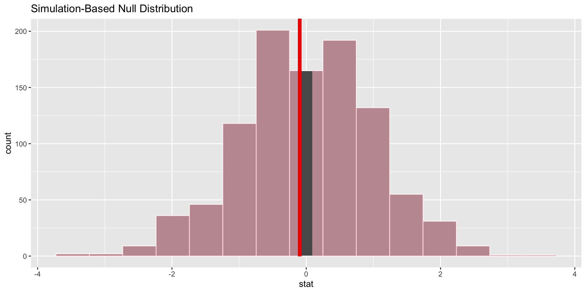
What did we end up with?

• A Z score for our sample!

test_stat$stat

[1] -0.09852599

• Interpretation: Our sample has a Z score of -0.1, meaning that it is .1 standard deviations below the mean of the null distribution. 0.1 standard deviations is a very small difference, so it’s looking likely that we will fail to reject the null hypothesis that men and women obtain college degrees at the same rate!

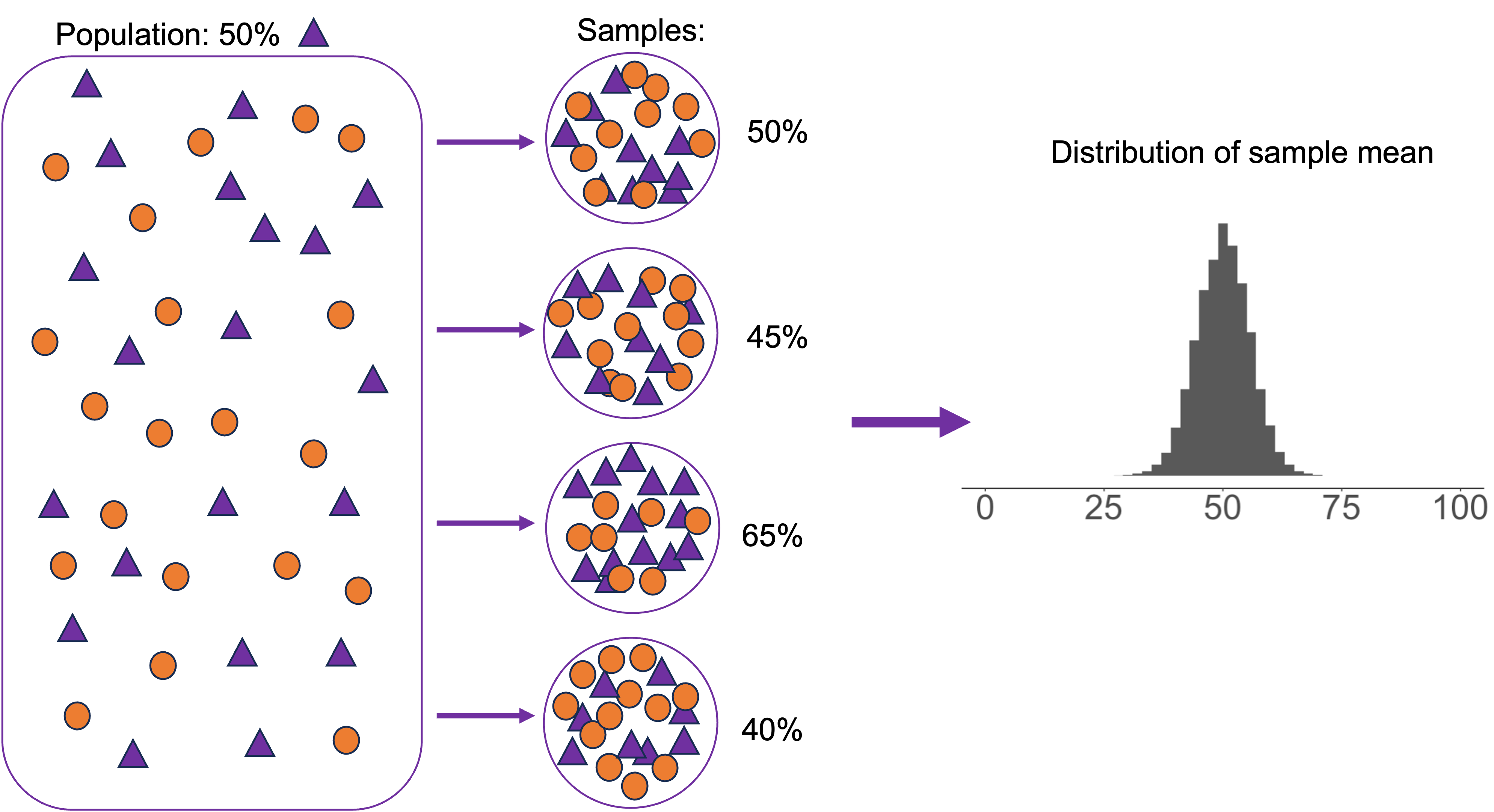
Step 2: Simulate the null distribution

• Now we have a test statistic for our sample. But we need to know what our null distribution looks like in order to turn that into a p value.
• Why? The p value is derived from the area in the tails of our null distribution, equal to or past the point where our sample is. So we need both the sample statistic (which we calculated in step 1) and the null distribution in order to find it.

Step 2: Simulate the null distribution with generate()

• This code is actually the same as the code we used before to calculate the test statistic, with just one addition!

• The line with generate() is the only new thing here.

• Instead of calculating a test statistic for our one sample, here generate() is doing some computational wizardry to create a null distribution.

  • Basically, it’s simulating pulling a bunch of samples from the population we assume under the null hypothesis.

null_dist <- gss |> 
  specify(explanatory = sex,             # just like before, we specify variables
          response = college,
          success = "degree") |> 
  hypothesize(null = "independence") |>  # then tell R what our null hypothesis is
  generate(reps = 1000) |>               # this part is new! We draw samples from the null distribution
  calculate(stat = "z")                  # and then we calculate the test statistics of our draws--just like before

Step 2: Simulate the null distribution with generate()

• Conceptually: generate() is pulling all of those samples that create the null distribution!

Step 3: Calculate the p value of the sample

• We use get_p_value() for this

get_p_value(null_dist,               # The first argument is our null distribution
            obs_stat = test_stat,    # Then the test statistic we calculated
            direction = "two-sided") # direction is related to whether the test is one or two tailed

# A tibble: 1 × 1
  p_value
    <dbl>
1   0.992

• Interpretation: There is a 99.2% chance that under the null hypothesis we would have obtained a sample with at least as big a difference between men’s and women’s rates of obtaining college degrees as this one
• This is way bigger than 5%! We fail to reject the null hypothesis. Men and women in this data set get college degrees at about the same rate.

Step 4: Visualize where your sample is with respect to your null distribution

• This isn’t strictly necessary—we already have the p value and were able to make a decision about what to do with the null hypothesis—but it’s always clarifying to see the picture.

visualize(null_dist) +                    # this plots the null distribution
  shade_p_value(obs_stat = test_stat,     # and this marks where our sample is
                direction = "two-sided")  # everything more extreme in either direction is shaded red

Steps to running a hypothesis test with infer

1. Calculate the test statistic of your sample

   • with specify() (telling R what your variables are),
   • then hypothesize() (telling R what kind of null hypothesis you have),
   • then calculate() (calculating your test statistic)

2. Simulate the null distribution

   • exactly the same code as step 1, but with an added generate() step
   • here you are simulating pulling a bunch of samples from your null population in order to figure out what the null distribution of sample statistics would look like

3. Calculate the p value of your sample

   • with your null distribution, your test statistic, and get_p_value()

4. Visualize the test statistic of your sample alongside the null distribution

   • with visualize() and shade_p_value()

Exercise Q3: Run your first hypothesis test!

• How is someone’s gender identity related to their probability of being married?

  • Explanatory variable: gender; categorical with two categories
  • Response variable: married; categorical with two categories
  • Correct test: A two-sample Z test, just like the example

• Don’t forget to run the setup chunks first: they will install and load infer for you